1. Heisenberg Uncertainty Principle
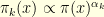
The Heisenberg Uncertainty principle states that a signal cannot be both highly concentrated in time and highly concentrated in frequency. For example, consider a square-integrable function  normalised so that
  . In this case,
  defines a probability distributions on the real line. The Fourier isometry shows that its Fourier transform
  also defines a probability distribution
  . In order to measure how spread-out these two probability distributions are, one can use their variance. The uncertainty principle states that

where  designates the variance of the distribution
  . This shows for example that
  and
and  cannot be simultaneously less than
  .
.
We can play the same with a vector  and its (discrete) Fourier transform
  . The Fourier matrix
  is defined by
where the normalisation coefficient  ensures that
  . The Fourier inversion formula reads
  . To measure how spread-out the coefficients of a vector
  are, one can look at the size of its support
![\displaystyle \mu(v) \, := \, \textbf{Card} \Big\{ k \in [1,N]: \; v_k=0 \Big\}. \ \ \ \ \ (3)](https://s0.wp.com/latex.php?latex=%5Cdisplaystyle++%5Cmu%28v%29+%5C%2C+%3A%3D+%5C%2C+%5Ctextbf%7BCard%7D+%5CBig%5C%7B+k+%5Cin+%5B1%2CN%5D%3A+%5C%3B+v_k%3D0+%5CBig%5C%7D.+%5C+%5C+%5C+%5C+%5C+%283%29&bg=ffffe3&fg=000000&s=0&c=20201002)
If an uncertainty principle holds, one should be able to bound  from below. There is no universal constant
  such that

for any  and . Indeed, if
  and
and  one readily checks that
  and
and  so that
  . Nevertheless, in this case this gives
  . Indeed, a beautiful result of L. Donoho and B. Stark shows that

Maybe more surprisingly, and crucial to applications, they even show that this principle can be made robust by taking noise and approximations into account. This is described in the next section.
2. Robust Uncertainty Principle
Consider a subset  of indices and the orthogonal projection
  on
on  . In other words, if
  , then

We say that a vector  is
is  -concentrated on
  if
if  . The
. The  -robust uncertainty principle states that if
  is concentrated on and
  is
is  -concentrated on
  then
then

Indeed, the case  gives Equation (5). The proof is surprisingly easy. On introduces the reconstruction operator
  defined by

In words: take a vector, delete the coordinate outside , take the Fourier transform, delete the coordinate outside , finally take the inverse Fourier transform. The special case  simply gives
  . The proof consists in bounding the operator norm of
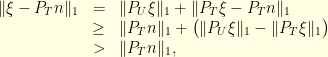
  from above and below. The existence of a vector that is -concentrated such that is -concentrated gives a lower bound. In details:
In summary, the reconstruction operator  always satisfies
  . Moreover, the existence of satisfying
  and
and  implies the lower bound
  . Therefore, the sets and must verify the uncertainty principle

Notice that we have only use the fact that the entries of the Fourier matrix are bounded in absolute value by . We could have use for example any other unitary matrix  . The bound
  for all
  gives the uncertainty principle
  . In general
  since
since  is an isometry.
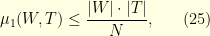
One can work out an upper bound and a lower bound for the reconstruction operator using the  -norm instead of the -norm. Doing so, one can prove that if
  and
and  then
then

3. Stable Reconstruction
Let us see how the uncertainty principle can be used to reconstruct a corrupted signal. For example, consider a discrete signal  corrupted by some noise
  . In top of that, let us suppose that on the set
  the receiver does not receive any information. In other words, the receiver can only observe

In general, it is impossible to recover the original  , or an approximation of it, since the data for
  are lost forever. In general, even if the received signal
  is very weak, the deleted data
  might be huge. Nevertheless, under the assumption that the frequencies of
  are supported by a set satisfying
  , the reconstruction becomes possible. It is not very surprising since the hypothesis implies that the signal
  is sufficiently smooth so that the knowledge of
  on
on  is enough to construct an approximation of for . We assume that the set is known to the observer. Since the components on are not observed, one can suppose without loss of generality that there is no noise on these components (
 we have
  for ): the observation
  can be described as

It is possible to have a stable reconstruction of the original signal if the operator  can be inverted: there exists a linear operator
  such that
  for every
  . If this is the case, the reconstruction
satisfies  so that
  . A sufficient condition for to exist is that
  for every . This is equivalent to

Since for we have  it follows that
  where is the reconstruction operator. The condition
  thus follows from the bound
  . Consequently the operator is invertible since
  satisfies

Since  we have the bound
  . Therefore

Notice also that  can easily and quickly be approximated using the expansion

Nevertheless, there are two things that are not very satisfying:
- the bound
 is extremely restrictive. For example, if
  of the component are corrupted, this imposes that the signal has only
  (and not
  ) non-zero Fourier coefficients.
- in general, the sets and are not known by the receiver.
The theory of compressed sensing addresses these two questions. More on that in forthcoming posts, hopefully … Emmanuel Candes recently gave extremely interesting lectures on compressed sensing.
4. Exact Reconstruction: Logan Phenomenon
Let us consider a slightly different situation. A small fraction of the components of a signal  are corrupted. The noise is not assumed to be small. More precisely, suppose that one observes

where is the set of corrupted components and  is an arbitrary noise that can potentially have very high intensity. Moreover, the set is unknown to the receiver. In general, it is indeed impossible to recover the original signal . Surprisingly, if one assumes that the signal is band-limited the Fourier transform of is supported by a known set that satisfies
it is possible to recover exactly the original . The main argument is that the condition (20) implies that the signal has more that  of its energy on
  in the sense that
  . Consequently, since is the set where the signal is perfectly known, enough information is available to recover the original signal . To prove the inequality , it suffices to check that
In this case we have  , which prove that has more that of its energy on . Indeed, the same conclusion holds with the -norm if the condition
  holds. The magic of the -norm is that condition
  implies that the signal is solution of the optimisation problem

This would not be true if one were using the norm instead. This idea was first discovered in a slightly different context in Logan’s thesis (1965). More details here. To prove (22), notice that any  can be written as
  with
with  . Therefore, since
  , it suffices to show that

This is equivalent to proving that for any non-zero we have

It is now that the -norm is crucial. Indeed, we have
which gives the conclusion. This would not work for any  -norm with
  since in general
  : the inequality is in the wrong sense. In summary, as soon as the condition
  is satisfied, one can recover the original signal by solving the minimisation problem (22).
\noindent Because it is not hard to check that in general we always have
this shows that the condition  implies that exact recovery is possible! Nevertheless, the condition
  is far from satisfying. The inequality is tight but in practice it happens very often that even if
  is much bigger that
  .
.
The take away message might be that perfect recovery is often possible if the signal has a sparse representation in an appropriate basis (in the example above, the usual Fourier Basis): the signal can then be recovered by -minimisation. For this to be possible, the representation basis (here the Fourier basis) must be incoherent with the observation basis in the sense that the coefficients of the change of basis matrix (here, Fourier matrix) must be small if  is the observation basis and
  is the representation basis then
  must be small for every
  . For example, for the Fourier basis we have
  for every .

black: observation basis, green:representation basis


 !? Easy you might say, that’s simply the hitting time of the state
  of the following Markov chain.
 is the expected number of steps before reaching
  is the expected number of steps before reaching
  ,
,  is the expected number of steps before reaching
  , etc… one can readily see that
  verify the system of equations
 . That was a little bit tedious and I don’t really want to know how long one should wait on average before observing the sequence
  .
. of length
  with
with  for all
  . To this end, one will introduce an army of gamblers, a casino, a game of chance and a martingale. The martingale
  describes the amount of money earned by the casino. At each round (starting at round
  ) the casino tosses a coin and the gamblers can make bets. If a gambler starts betting just before round
  . If he decides to bet again at round
  , he wins if the coin shows
  , etc… Suppose that there are infinitely many gamblers
  and that gambler
  starts betting just before round
  he gets
  and with probability
  dollar just before round
  ). Indeed, the amount of money earned by the casino is a martingale and
  . For example,
  if the first gambler
  loses his bet and
  if the wins. Consider the time
  when the magic coin pattern first appears. This is a stopping time and the optional stopping theorem for martingales shows that
 ![{\mathbb{E}[M_{\tau}] = 0}](https://s0.wp.com/latex.php?latex=%7B%5Cmathbb%7BE%7D%5BM_%7B%5Ctau%7D%5D+%3D+0%7D&bg=ffffe3&fg=000000&s=0&c=20201002) . Indeed, one can also compute this quantity another way. By time
. Indeed, one can also compute this quantity another way. By time  . in other words,
 if the gambler
  is still in the game after the round
  otherwise. The fundamental remark is that the quantity
  is not random so that
 ![{\mathbb{E}[\tau] = \sum_{j=0}^{\tau-1} 2^{\tau-k} \, \delta_j}](https://s0.wp.com/latex.php?latex=%7B%5Cmathbb%7BE%7D%5B%5Ctau%5D+%3D+%5Csum_%7Bj%3D0%7D%5E%7B%5Ctau-1%7D+2%5E%7B%5Ctau-k%7D+%5C%2C+%5Cdelta_j%7D&bg=ffffe3&fg=000000&s=0&c=20201002) . Indeed, right after round
. Indeed, right after round  is still in the game or not. Gambler
  is in the game only if the
  then the gamblers who have seen the pattern
  and
and ![{\mathbb{E}[\tau] = 2^1+2^4+2^7}](https://s0.wp.com/latex.php?latex=%7B%5Cmathbb%7BE%7D%5B%5Ctau%5D+%3D+2%5E1%2B2%5E4%2B2%5E7%7D&bg=ffffe3&fg=000000&s=0&c=20201002) .
.
 coin tosses before observing the pattern
  extracted from a recent
  dimensional Brownian motion
  . Suppose that
  is an
is an  to
to  with boundary
 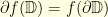 where
where  . A two dimensional brownian motion started at
  takes on average
![\displaystyle \mathbb{E}[ \, \tau \, ] \; = \; \sum_{k \geq 1} |a_k|^2](https://s0.wp.com/latex.php?latex=%5Cdisplaystyle+%5Cmathbb%7BE%7D%5B+%5C%2C+%5Ctau+%5C%2C+%5D+%5C%3B+%3D+%5C%3B+%5Csum_%7Bk+%5Cgeq+1%7D+%7Ca_k%7C%5E2+&bg=ffffe3&fg=000000&s=0&c=20201002)
 and
and  is the
  . Indeed, since the situation is invariant by translation one can always suppose that
  . The proof of this result is a simple martingale argument. Indeed, since
  is a martingale, the
 ![\displaystyle \mathbb{E}[ \, \|B_{\tau}\|^2 \, ] \; = \; 2 \mathbb{E}[\, \tau \, ].](https://s0.wp.com/latex.php?latex=%5Cdisplaystyle+%5Cmathbb%7BE%7D%5B+%5C%2C+%5C%7CB_%7B%5Ctau%7D%5C%7C%5E2+%5C%2C+%5D+%5C%3B+%3D+%5C%3B+2+%5Cmathbb%7BE%7D%5B%5C%2C+%5Ctau+%5C%2C+%5D.+&bg=ffffe3&fg=000000&s=0&c=20201002)
 is an analytic function,
  , up to a time change, where
  is another
  . Consequently,
  where
where  is the hitting time
  . This shows that
![\displaystyle \mathbb{E}[ \, \|B_{\tau}\|^2 \, ] = \mathbb{E}[ \, \|f(W_{\rho})\|^2 \, ] = \frac{1}{2\pi} \int_{\theta=0}^{2\pi} |f(e^{i\theta})|^2 \, d\theta.](https://s0.wp.com/latex.php?latex=%5Cdisplaystyle+%5Cmathbb%7BE%7D%5B+%5C%2C+%5C%7CB_%7B%5Ctau%7D%5C%7C%5E2+%5C%2C+%5D+%3D+%5Cmathbb%7BE%7D%5B+%5C%2C+%5C%7Cf%28W_%7B%5Crho%7D%29%5C%7C%5E2+%5C%2C+%5D+%3D+%5Cfrac%7B1%7D%7B2%5Cpi%7D+%5Cint_%7B%5Ctheta%3D0%7D%5E%7B2%5Cpi%7D+%7Cf%28e%5E%7Bi%5Ctheta%7D%29%7C%5E2+%5C%2C+d%5Ctheta.+&bg=ffffe3&fg=000000&s=0&c=20201002)
 , the conclusion follows.
![{\mathbb{E}[ \, \tau \, ]}](https://s0.wp.com/latex.php?latex=%7B%5Cmathbb%7BE%7D%5B+%5C%2C+%5Ctau+%5C%2C+%5D%7D&bg=ffffe3&fg=000000&s=0&c=20201002) . The first thing that comes to mind is a strip
. The first thing that comes to mind is a strip  since it is classical that a Brownian motion started at
  to exit the strip
  . Since
  maps the unit disk
  it follows that
 .
. and suppose that each point
  represents a city. Each city is connected to its
  neighbors only and each edge
  carries a weight that represents the time it takes to go from city
  . In other words, each edge of the lattice
  . The random variables
  are
are  and distributed according to
 hours, say. On the next picture, each red dot represents a city that can be reached in less than
 cities (the origin is the blue dotted city) and highlighted the optimal routes between the origin and each one of the cities on the border of the map.


 and a
and a  . How does it look like ? What is the invariant distribution ?
![{D=[0,1] \subset \mathbb{R}}](https://s0.wp.com/latex.php?latex=%7BD%3D%5B0%2C1%5D+%5Csubset+%5Cmathbb%7BR%7D%7D&bg=ffffe3&fg=000000&s=0&c=20201002) . In other words, what does a real Brownian motion conditioned to stay inside the segment
. In other words, what does a real Brownian motion conditioned to stay inside the segment ![{[0,1]}](https://s0.wp.com/latex.php?latex=%7B%5B0%2C1%5D%7D&bg=ffffe3&fg=000000&s=0&c=20201002) look like.
look like. and a standard random walk
  : with probability
  the random walk goes up
  and with probability
  . For clarity, assume that there exists an integer
  such that
  . Suppose as well that it is conditioned on the event
 ![{X_k \in [0,1]}](https://s0.wp.com/latex.php?latex=%7BX_k+%5Cin+%5B0%2C1%5D%7D&bg=ffffe3&fg=000000&s=0&c=20201002) for
for  . Later, we will consider the limiting case
  and
and  , in this order, to recover the Brownian motion case.
 conditioned on the event
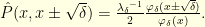
  . This is a Doob
 ![{\hat{P}(k,x,y) = \mathbb{P}[\hat{X}_{k+1}=y \,|\hat{X}_k=x]}](https://s0.wp.com/latex.php?latex=%7B%5Chat%7BP%7D%28k%2Cx%2Cy%29+%3D+%5Cmathbb%7BP%7D%5B%5Chat%7BX%7D_%7Bk%2B1%7D%3Dy+%5C%2C%7C%5Chat%7BX%7D_k%3Dx%5D%7D&bg=ffffe3&fg=000000&s=0&c=20201002) with
with  where
where ![{D_{\delta} = \sqrt{\delta} \mathbb{N} \; \cap \; [0,1]}](https://s0.wp.com/latex.php?latex=%7BD_%7B%5Cdelta%7D+%3D+%5Csqrt%7B%5Cdelta%7D+%5Cmathbb%7BN%7D+%5C%3B+%5Ccap+%5C%3B+%5B0%2C1%5D%7D&bg=ffffe3&fg=000000&s=0&c=20201002) . One can compute the probability that the conditioned Markov chain follows a given trajectory
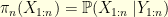
. One can compute the probability that the conditioned Markov chain follows a given trajectory  of
of  ,
,![\displaystyle \begin{array}{rcl} \mathbb{P}[\hat{X}_0 = x_0, \ldots, \hat{X}_N=x_N] = \frac{1}{Z(N,\delta)} P(x_0,x_1) \times \ldots \times P(x_{N-1}, x_N) \end{array}](https://s0.wp.com/latex.php?latex=%5Cdisplaystyle++%5Cbegin%7Barray%7D%7Brcl%7D++%5Cmathbb%7BP%7D%5B%5Chat%7BX%7D_0+%3D+x_0%2C+%5Cldots%2C+%5Chat%7BX%7D_N%3Dx_N%5D+%3D+%5Cfrac%7B1%7D%7BZ%28N%2C%5Cdelta%29%7D+P%28x_0%2Cx_1%29+%5Ctimes+%5Cldots+%5Ctimes+P%28x_%7BN-1%7D%2C+x_N%29+%5Cend%7Barray%7D+&bg=ffffe3&fg=000000&s=0&c=20201002)
 is the
 ![{Z(N,\delta) = \mathbb{P}[X_k \in D_{\delta} \; \text{for} \; k=0, \ldots, N]}](https://s0.wp.com/latex.php?latex=%7BZ%28N%2C%5Cdelta%29+%3D+%5Cmathbb%7BP%7D%5BX_k+%5Cin+D_%7B%5Cdelta%7D+%5C%3B+%5Ctext%7Bfor%7D+%5C%3B+k%3D0%2C+%5Cldots%2C+N%5D%7D&bg=ffffe3&fg=000000&s=0&c=20201002) is a normalisation constant. The Doob
is a normalisation constant. The Doob ![\displaystyle \begin{array}{rcl} \mathbb{P}[\hat{X}_0 = x_0, \ldots, \hat{X}_N=x_N] = \hat{P}(0,x_0,x_1) \times \ldots \times \hat{P}(N-1,x_{N-1}, x_N) \end{array}](https://s0.wp.com/latex.php?latex=%5Cdisplaystyle++%5Cbegin%7Barray%7D%7Brcl%7D++%5Cmathbb%7BP%7D%5B%5Chat%7BX%7D_0+%3D+x_0%2C+%5Cldots%2C+%5Chat%7BX%7D_N%3Dx_N%5D+%3D+%5Chat%7BP%7D%280%2Cx_0%2Cx_1%29+%5Ctimes+%5Cldots+%5Ctimes+%5Chat%7BP%7D%28N-1%2Cx_%7BN-1%7D%2C+x_N%29+%5Cend%7Barray%7D+&bg=ffffe3&fg=000000&s=0&c=20201002)
 and the function
  is defined by
![\displaystyle \begin{array}{rcl} h(k,x) = \mathbb{P}[X_{j} \in D_{\delta} \; \text{for} \; k+1 \leq j \leq N \, |X_k=x]. \end{array}](https://s0.wp.com/latex.php?latex=%5Cdisplaystyle++%5Cbegin%7Barray%7D%7Brcl%7D++h%28k%2Cx%29+%3D+%5Cmathbb%7BP%7D%5BX_%7Bj%7D+%5Cin+D_%7B%5Cdelta%7D+%5C%3B+%5Ctext%7Bfor%7D+%5C%3B+k%2B1+%5Cleq+j+%5Cleq+N+%5C%2C+%7CX_k%3Dx%5D.+%5Cend%7Barray%7D+&bg=ffffe3&fg=000000&s=0&c=20201002)
 for all
  . The quantity
  is the probability that a random walk starting at
  . Consequently, in order to find the transition probabilities of the conditioned kernel, it suffices to compute the quantities
  for all
  . It can be computed recursively since
  with the appropriate boundary conditions. In other words, adopting the obvious matrix notations, the vector
  satisfies
 is the usual tridiagonal matrix given by
  if, and only if,
  and
and  otherwise. It is related to the
  where
where  is the highest eigenvalue of
  the associated eigenfunction. The eigenvalues of
 ![{D=[0,1]}](https://s0.wp.com/latex.php?latex=%7BD%3D%5B0%2C1%5D%7D&bg=ffffe3&fg=000000&s=0&c=20201002) with
with  and
and
 . To obtain the dynamics of the conditioned Brownian motion it suffices to consider the limiting case

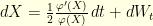 where
where  is the first eigenfunction of the Laplacian on
 is the first eigenfunction of the Laplacian on
![{D=[0,1]^2 \subset \mathbb{R}^2}](https://s0.wp.com/latex.php?latex=%7BD%3D%5B0%2C1%5D%5E2+%5Csubset+%5Cmathbb%7BR%7D%5E2%7D&bg=ffffe3&fg=000000&s=0&c=20201002) .
.
 since
since  are isometries and
  are orthogonal projections. Moreover, the smaller
  is an isometry we have
  , where the supremum is over all
  that are supported by
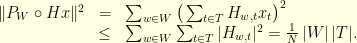
 .
. and
and  . The Fourier transform is an
  in the sense that


 ‘s by
‘s by  be a Markov kernel on a metric state space
  . We would like to quantify how long it takes for two different particles evolving according to the Markovian dynamic given by
  and the second at
  , the initial distance between them is
  . At time
  , what is the average distance between these two particles. For example, if
  and
and  are two Brownian motions in
  started from
  and
and  should be closer from each other than
  and
and  . Indeed, one can even show that whatever the coupling of these two Brownian motions we have
 ![{\mathop{\mathbb E}[d(W^x_t, W^y_t)] \geq d(x,y)}](https://s0.wp.com/latex.php?latex=%7B%5Cmathop%7B%5Cmathbb+E%7D%5Bd%28W%5Ex_t%2C+W%5Ey_t%29%5D+%5Cgeq+d%28x%2Cy%29%7D&bg=ffffe3&fg=000000&s=0&c=20201002) : this is roughly speaking because the Euclidean space
: this is roughly speaking because the Euclidean space  defined by
 of the space
  and develop a notion of curvature, we use the
  between probability measures. It is defined as
![{\mu(f) - \nu(f) = \mathop{\mathbb E}[f(X) - f(Y)]}](https://s0.wp.com/latex.php?latex=%7B%5Cmu%28f%29+-+%5Cnu%28f%29+%3D+%5Cmathop%7B%5Cmathbb+E%7D%5Bf%28X%29+-+f%28Y%29%5D%7D&bg=ffffe3&fg=000000&s=0&c=20201002) for any coupling
for any coupling  of
of  and
and  , and since the function
  is
is ![{\mathop{\mathbb E}[f(X) - f(Y)] \leq \mathop{\mathbb E}[d(X,Y)]}](https://s0.wp.com/latex.php?latex=%7B%5Cmathop%7B%5Cmathbb+E%7D%5Bf%28X%29+-+f%28Y%29%5D+%5Cleq+%5Cmathop%7B%5Cmathbb+E%7D%5Bd%28X%2CY%29%5D%7D&bg=ffffe3&fg=000000&s=0&c=20201002) . Consequently, for any coupling
. Consequently, for any coupling ![{W(\mu,\nu) \leq \mathop{\mathbb E}[d(X,Y)]}](https://s0.wp.com/latex.php?latex=%7BW%28%5Cmu%2C%5Cnu%29+%5Cleq+%5Cmathop%7B%5Cmathbb+E%7D%5Bd%28X%2CY%29%5D%7D&bg=ffffe3&fg=000000&s=0&c=20201002) . Taking the infimum over all the couplings
. Taking the infimum over all the couplings ![\displaystyle W(\mu,\nu) \;=\; \sup_{\text{Lip}(f) \leq 1} \; |\mu(f) - \nu(f)| \;\leq\; \inf_{(X,Y)} \; \mathop{\mathbb E}[d(X,Y)]. \ \ \ \ \ (3)](https://s0.wp.com/latex.php?latex=%5Cdisplaystyle++W%28%5Cmu%2C%5Cnu%29+%5C%3B%3D%5C%3B+%5Csup_%7B%5Ctext%7BLip%7D%28f%29+%5Cleq+1%7D+%5C%3B+%7C%5Cmu%28f%29+-+%5Cnu%28f%29%7C+%5C%3B%5Cleq%5C%3B+%5Cinf_%7B%28X%2CY%29%7D+%5C%3B+%5Cmathop%7B%5Cmathbb+E%7D%5Bd%28X%2CY%29%5D.+%5C+%5C+%5C+%5C+%5C+%283%29&bg=ffffe3&fg=000000&s=0&c=20201002)
![\displaystyle W(\mu,\nu) \;=\; \sup_{\text{Lip}(f) \leq 1} \; |\mu(f) - \nu(f)| \;=\; \inf_{(X,Y)} \; \mathop{\mathbb E}[d(X,Y)]. \ \ \ \ \ (4)](https://s0.wp.com/latex.php?latex=%5Cdisplaystyle+++W%28%5Cmu%2C%5Cnu%29+%5C%3B%3D%5C%3B+%5Csup_%7B%5Ctext%7BLip%7D%28f%29+%5Cleq+1%7D+%5C%3B+%7C%5Cmu%28f%29+-+%5Cnu%28f%29%7C+%5C%3B%3D%5C%3B+%5Cinf_%7B%28X%2CY%29%7D+%5C%3B+%5Cmathop%7B%5Cmathbb+E%7D%5Bd%28X%2CY%29%5D.+%5C+%5C+%5C+%5C+%5C+%284%29&bg=ffffe3&fg=000000&s=0&c=20201002)
 the one step distribution of the Markov chain started from
 ![{m_x(A) = \mathop{\mathbb P}[X_1 \in A \;| X_0 = x ]}](https://s0.wp.com/latex.php?latex=%7Bm_x%28A%29+%3D+%5Cmathop%7B%5Cmathbb+P%7D%5BX_1+%5Cin+A+%5C%3B%7C+X_0+%3D+x+%5D%7D&bg=ffffe3&fg=000000&s=0&c=20201002) , we define the local (Ricci) curvature
, we define the local (Ricci) curvature  between
 , the more the trajectories started at
 is strictly positive,
 for all neighbouring states
  . This can be proved thanks to the so called Gluing Lemma. A space without curvature correspond to the case
  : for example, a symmetric random walk on
  and a Brownian motion on
  have both zero curvature. The curvature
  is a property of both the metric space
  as the largest real number
  and
and  we have
 small enough. The quantity
  is the distribution of
  when started from
 ![{m_x^{\delta}(A) = \mathop{\mathbb P}[X_{\delta} \in A \; |X_0=x]}](https://s0.wp.com/latex.php?latex=%7Bm_x%5E%7B%5Cdelta%7D%28A%29+%3D+%5Cmathop%7B%5Cmathbb+P%7D%5BX_%7B%5Cdelta%7D+%5Cin+A+%5C%3B+%7CX_0%3Dx%5D%7D&bg=ffffe3&fg=000000&s=0&c=20201002) .
. for any
  in the sense that
 of
of  and
and  such that
 ![{W(m_x,m_y)=\mathop{\mathbb E}[d(U_{x,y}, V_{x,y})]}](https://s0.wp.com/latex.php?latex=%7BW%28m_x%2Cm_y%29%3D%5Cmathop%7B%5Cmathbb+E%7D%5Bd%28U_%7Bx%2Cy%7D%2C+V_%7Bx%2Cy%7D%29%5D%7D&bg=ffffe3&fg=000000&s=0&c=20201002) . Now, choose an optimal coupling
. Now, choose an optimal coupling  is a coupling (in general not optimal) of
  and
and  so that
![\displaystyle \begin{array}{rcl} W(\mu P, \nu P) &\leq& \mathop{\mathbb E}[d(U_{X,Y}, V_{X,Y})] = \mathop{\mathbb E}[\; \mathop{\mathbb E}[d(U_{x,y}, V_{x,y}) \;|X=x, Y=y] ] \\ &=& \mathop{\mathbb E}[ W(m_X, m_Y) ] = \mathop{\mathbb E}[ d(X,Y) \cdot (1-\kappa(X,Y)) ]\\ &\leq& (1-\kappa) \; \mathop{\mathbb E}[ d(X,Y) ] = (1-\kappa) \; W(\mu,\nu). \end{array}](https://s0.wp.com/latex.php?latex=%5Cdisplaystyle++%5Cbegin%7Barray%7D%7Brcl%7D++W%28%5Cmu+P%2C+%5Cnu+P%29+%26%5Cleq%26+%5Cmathop%7B%5Cmathbb+E%7D%5Bd%28U_%7BX%2CY%7D%2C+V_%7BX%2CY%7D%29%5D+%3D+%5Cmathop%7B%5Cmathbb+E%7D%5B%5C%3B+%5Cmathop%7B%5Cmathbb+E%7D%5Bd%28U_%7Bx%2Cy%7D%2C+V_%7Bx%2Cy%7D%29+%5C%3B%7CX%3Dx%2C+Y%3Dy%5D+%5D+%5C%5C+%26%3D%26+%5Cmathop%7B%5Cmathbb+E%7D%5B+W%28m_X%2C+m_Y%29+%5D+%3D+%5Cmathop%7B%5Cmathbb+E%7D%5B+d%28X%2CY%29+%5Ccdot+%281-%5Ckappa%28X%2CY%29%29+%5D%5C%5C+%26%5Cleq%26+%281-%5Ckappa%29+%5C%3B+%5Cmathop%7B%5Cmathbb+E%7D%5B+d%28X%2CY%29+%5D+%3D+%281-%5Ckappa%29+%5C%3B+W%28%5Cmu%2C%5Cnu%29.+%5Cend%7Barray%7D+&bg=ffffe3&fg=000000&s=0&c=20201002)


 . In continuous time, this reads
 that is uniformly elliptic in the sense
  . The Langevin diffusion
 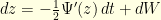 has invariant distribution
  . Given a time step
 . Given two starting points
  and
and  , using the same noise
  to define
  and
and  it immediately follows that
 is positively curved with curvature (at least) equal to
  .
. on this unit sphere: by symmetry, one can always rotate the coordinates so that that
  and
and 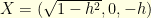 for some
 ![{h \in [0,1]}](https://s0.wp.com/latex.php?latex=%7Bh+%5Cin+%5B0%2C1%5D%7D&bg=ffffe3&fg=000000&s=0&c=20201002) . For
. For  the (geodesic) distance
  is approximated by
  . One can couple two Brownian motions
  and
and  , one started at
  and the other one started at
  , by the usual symmetry with respect to the plane
  : in other words,
  . One can check (good exercise!) that the diffusion followed by the
  -coordinate of a Brownian motion on the unit sphere of
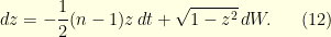
 , it follows that
 and
and  since
since  it readily follows that
 . Maybe surprisingly, the higher the dimension, the faster the convergence to equilibrium. This is not so unreal if one notices that the Brownian increment satisfies
  .
.
 numbers lying at the bottom, and each one of them is an integer between
  : these numbers must be different so that there are at most
  possibilities to test! Brute force won’t work my friend!
 such that a solution to the problem corresponds to a low energy configuration, one can do MCMC-simulating annealing-etc on the target distribution
 . Foolishly, I first tried the following energy function, and then ran a random walk
 is the numbers of levels that one can fill, starting from the bottom, without encountering any problem
  no repetition and no number greater than
  and letting run the algorithm for a few millions iterations (
 min on my crappy laptop), one can easily produce configurations that are
  and
and  and
and  . This conditioned Markov chain
  is still a
  of the unconditioned Markov chain, which are usually not available: this has been discussed in this previous
  with transition operator
  is
is 
 is equal to
  , which is also equal to
  if the chain is reversible.
![{[a,b]}](https://s0.wp.com/latex.php?latex=%7B%5Ba%2Cb%5D%7D&bg=ffffe3&fg=000000&s=0&c=20201002) . Indeed, the situation is completely different in higher dimensions.
. Indeed, the situation is completely different in higher dimensions. , that has
  or
or  is reversible: such a Markov chain is usually called skip-free in the litterature. This is extremely easy to prove, and since skip-free Markov chains have been studied a lot, I am sure that this result is somewhere in the litterature (any reference for that?). To show the result, it suffices to show that
  for any
  where
where  is the upward flux at level
  is the downward flux. Because
 . Interating we get that for any
  we have
  : the conclusion follows since
  .
. since under regularity assumptions on
  and
and  they can be seen as limit of skip-free one dimensional Markov chains on
  . Indeed, I guess that the usual proof of this result goes through introducing the scale function and the speed measure of the diffusion, but I would be very glad if anyone had another pedestrian approach that gives more intuition into this.
 between
  and
and  , starting from
 between
![{t \in [0,T]}](https://s0.wp.com/latex.php?latex=%7Bt+%5Cin+%5B0%2CT%5D%7D&bg=ffffe3&fg=000000&s=0&c=20201002) such that
such that  then define the path
 ![\displaystyle X^{\star}_s = \left\{ \begin{array}{ll} X^{(a)}_s & \text{ for } s \in [0,t]\\ X^{(b)}_s & \text{ for } s \in [t,T], \end{array} \right. \ \ \ \ \ (2)](https://s0.wp.com/latex.php?latex=%5Cdisplaystyle++X%5E%7B%5Cstar%7D_s+%3D+%5Cleft%5C%7B+%5Cbegin%7Barray%7D%7Bll%7D+X%5E%7B%28a%29%7D_s%09%26+%5Ctext%7B+for+%7D+s+%5Cin+%5B0%2Ct%5D%5C%5C+X%5E%7B%28b%29%7D_s%09%26+%5Ctext%7B+for+%7D+s+%5Cin+%5Bt%2CT%5D%2C+%5Cend%7Barray%7D+%5Cright.+%5C+%5C+%5C+%5C+%5C+%282%29&bg=ffffe3&fg=000000&s=0&c=20201002) and otherwise go back to step
and otherwise go back to step  and
and  , with parameter
  .
.
 such that
