The other day, Nathanael Berestycki presented some very nice results on random permutations. Start with the identity permutation of  and compose with random transpositions: in short, at time
  we consider the random permutation
  where
where  is a transposition chosen uniformly at random among the
  transpositions of . How long do we have to wait before seeing a permutation that has a cycle of length greater than
  , where
  is a fixed constant ?
The answer has been known for quite a long time (O. Schramm,2005), but no simple proof was available: the highlight of Nathanael’s talk was a short and elegant proof of the fact that we only have to wait a little bit more than  steps to see this giant cycle! The first half of the proof is such a beauty that I cannot resist in sharing it here!
1. Visual representation
First, this is more visual to represent a permutation by its cycle decomposition. Consider for example the permutation  that sends
  etc… It can be graphically represented by the following pictures:

cycle structure - visual representation
If this permutation is composed with the transposition  , this gives the following cycle structure:

two cycles merge
If it is composed with  this gives,

a cycles breaks down into two
It is thus pretty clear that the cycle structure of  can be obtained from the cycle structure of
  in only 2 ways:
- or two cycles of merge into one,
- or one cycle of breaks into two cycles.
In short, the process  behaves like a fragmentation-coalescence processes. At the beginning, the cycle structure of
  is trivial: there are
  trivial cycles of length one! Then, as times goes by, they begin to merge, and sometimes they also break down. At each step two integers
  and
and  are chosen uniformly at random (with
  ): if and belong to the same cycle, this cycle breaks into two parts. Otherwise the cycle that contains merges with the cycle that contains . Of course, since at the beginning all the cycles are extremely small, the probability that a cycles breaks into two part is extremely small: a cycle of size breaks into two part with probability roughly equal to
  .
.
2. Comparison with the Erdos-Renyi random Graph
Since the fragmentation part of the process can be neglected at the beginning, this is natural to compare the cycle structure at time with the rangom graph  where
where  : this graph has vertices and roughly edges since each vertex is open with probability
  . A coupling argument makes this idea more precise:
- start with
 and the graph
  that has disconnected vertices
- choose two different integers
- define

- to define
 , take
  and join the vertices and (never mind if they were already joined)
- go to step
 .
.
The fundamental remark is that each cycle of is included in a connected component of : this is true at the beginning, and this property obviously remains true at each step. The Erdos-Renyi random graph  is one of the most studied object: it is well-known that for
  , with probability tending to
  , the size of the largest connected component of
  is of order
  . Since
  , this immediately shows that for
  , with
  the length of the longuest cycle in is of order or less. This is one half of the result. It remains to work a little bit to show that if we wait a little bit more than
  , the first cycle of order appears.
For a permutation  with cycle decomposition
  (cycles of length included), one can consider the quantity
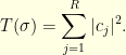
This is a quantity between (for the identity) and  that measures in some extends the sizes of the cycles. In order to normalize everything and to take into account that the cycle structure abruptly changes near the critical value , one can also observe this quantity on a logarithmic scale:

This quantity  lies between
  and , and evolves quite smoothly with time: look at what it looks like, once the time has been rescaled by a factor :

fluid limit ?
The plot represented the evolution of the quantity  between time
  and
and  for dimensions
  .
.
Question: does the random quantity  converge (in probability) towards a non trivial constant
  ? It must be the analogue quantity for the random graph
  , so I bet it is a known result …


