The other day Christina Goldschmidt gave a very nice talk on results obtained by James Norris and R. W. R. Darling: in their paper they use fluid limit techniques in order to study properties a Random graphs. This approach has long been used to analyse queuing systems for example.
1. Erdos Renyi Random Graph model
Remember that the Erdos Renyi random graph  is a graph with
  vertices
  such that any two of them are connected with probability
  , independently.

Erdos-Renyi random graph model
This model of random graphs has been extensively studied and this has long been known that  undergoes a phase transition at
  : for
: for  , the largest component
  of
of  has a size of order
  while for
  the largest connected component , also called the giant component, has size of order . In another blog entry, another consequence of this phase transition has been used.
One can even show that for there exists a constant  such that for any
  ,
,

Simply put, the largest connected component of has size approximatively equal to  . Maybe surprisingly, this is quite simple to compute the value of
  through fluid limit techniques.
2. Exploration of the graph
Let  be a configuration of
  . This configuration is explored through a classical depth-first algorithm. To keep track of what is doing, a process
  is introduced. This process captures essentially all the information needed to study the size of the connected component: it is then shown that
  behaves essentially deterministically when looked under the appropriate scale.
- initilisation: t=0: Color all the vertices in green, the current vertex is
 and define
  .
.
- t=t+1: Color the current vertex in red (=visited): if a vertex is connected to
 and is green, color it in grey ( this vertex has still to be visited, but its ‘parent’ has already been visited): these are the children of .
- update the following way,
 , and
, and
- if has children, choose one of them and make it the new current vertex. Go to
 .
.
- If has no children then the new current vertex is its parent. Go to .
- if has no children and no parent, the new current vertex is one of the remaining (if any) green vertex. Go to
- else: we are finished.

A moment of though reveals that and reaches  precisely when the connected component of the vertex
  has all been explored. Then reaches
  precisely when the second connected component has all been explored, etc … This is why if
  and
and  then the connected components have size exactly
  for
for  . The largest component has size
  .
.

Z process
3. Fluid Limit
It is quite easy to show why the rescaled process ![{z^N(t) = \frac{ Z([Nt])}{N}}](https://s0.wp.com/latex.php?latex=%7Bz%5EN%28t%29+%3D+%5Cfrac%7B+Z%28%5BNt%5D%29%7D%7BN%7D%7D&bg=ffffe3&fg=000000&s=0&c=20201002) should behave like a differential equation (ie: fluid limit). While exploring the first component,
should behave like a differential equation (ie: fluid limit). While exploring the first component,  represents the number of gray vertices at time
  so that
  represents the number of green vertices: this is why
![\displaystyle \mathop{\mathbb E}\Big[Z_{k+1}-Z_k \;|Z_k \Big] = (N-k-Z_k) \frac{c}{N} = c\Big(1-\frac{k}{N} - \frac{Z_k}{N} \Big) - 1](https://s0.wp.com/latex.php?latex=%5Cdisplaystyle++%5Cmathop%7B%5Cmathbb+E%7D%5CBig%5BZ_%7Bk%2B1%7D-Z_k+%5C%3B%7CZ_k+%5CBig%5D+%3D+%28N-k-Z_k%29+%5Cfrac%7Bc%7D%7BN%7D+%3D+c%5CBig%281-%5Cfrac%7Bk%7D%7BN%7D+-+%5Cfrac%7BZ_k%7D%7BN%7D+%5CBig%29+-+1&bg=ffffe3&fg=000000&s=0&c=20201002)
so that ![{\mathop{\mathbb E}\Big[ \frac{z^N(t+\Delta)-z^N(t)}{\Delta} | z^N(t) \Big] \approx c\Big(1-t-z(t) \Big) - 1}](https://s0.wp.com/latex.php?latex=%7B%5Cmathop%7B%5Cmathbb+E%7D%5CBig%5B+%5Cfrac%7Bz%5EN%28t%2B%5CDelta%29-z%5EN%28t%29%7D%7B%5CDelta%7D+%7C+z%5EN%28t%29+%5CBig%5D+%5Capprox+c%5CBig%281-t-z%28t%29+%5CBig%29+-+1%7D&bg=ffffe3&fg=000000&s=0&c=20201002) where
where  . Also, the variance statisfies
 ![{\text{Var}\Big[ \frac{z^N(t+\Delta)-z^N(t)}{\sqrt{\Delta}} | z^N(t) \Big] \approx N^{-\frac{1}{2}} c\Big(1-t-z(t) \Big) \rightarrow 0}](https://s0.wp.com/latex.php?latex=%7B%5Ctext%7BVar%7D%5CBig%5B+%5Cfrac%7Bz%5EN%28t%2B%5CDelta%29-z%5EN%28t%29%7D%7B%5Csqrt%7B%5CDelta%7D%7D+%7C+z%5EN%28t%29+%5CBig%5D+%5Capprox+N%5E%7B-%5Cfrac%7B1%7D%7B2%7D%7D+c%5CBig%281-t-z%28t%29+%5CBig%29+%5Crightarrow+0%7D&bg=ffffe3&fg=000000&s=0&c=20201002) so that all the ingredients for a fluit limit are present:
so that all the ingredients for a fluit limit are present:  converges to the differential equation
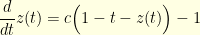
whose solution is 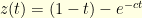 . This is why
  is implicitly defined as the solution of
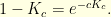
As expected,  and
and  .
.


