
Brownian Motion
A few days ago, a student asked the following question:
Consider a bounded domain  and a Brownian motion conditioned to stay inside
  . How does it look like ? What is the invariant distribution ?
This is very simple, and surprisingly interesting. This involves the first eigenfunction of the Laplacian on . To make everything simple, and because this does not change anything, it suffices to study the situation where ![{D=[0,1] \subset \mathbb{R}}](https://s0.wp.com/latex.php?latex=%7BD%3D%5B0%2C1%5D+%5Csubset+%5Cmathbb%7BR%7D%7D&bg=ffffe3&fg=000000&s=0&c=20201002) . In other words, what does a real Brownian motion conditioned to stay inside the segment
. In other words, what does a real Brownian motion conditioned to stay inside the segment ![{[0,1]}](https://s0.wp.com/latex.php?latex=%7B%5B0%2C1%5D%7D&bg=ffffe3&fg=000000&s=0&c=20201002) look like.
look like.
Discretisation
One could directly do the computations in a continuous setting but, as it is often the case, it is simpler to consider the usual random walk discretisation of a Brownian motion. For this purpose, consider a time discretisation  and a standard random walk
  with increment
  : with probability
  the random walk goes up
  and with probability it goes down
  . For clarity, assume that there exists an integer
  such that
  . Suppose as well that it is conditioned on the event
 ![{X_k \in [0,1]}](https://s0.wp.com/latex.php?latex=%7BX_k+%5Cin+%5B0%2C1%5D%7D&bg=ffffe3&fg=000000&s=0&c=20201002) for
for  . Later, we will consider the limiting case
  and
and  , in this order, to recover the Brownian motion case.
Conditioning
First, let us compute the probability transitions of the random walk  conditioned on the event for . For clarity, let us denote the conditioned random walk by
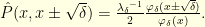
  . This is a Doob h-transform, and the resulting process is a non-homogenous Markov chain. In this simple case the computations are straightforward. The conditioned Markov chain has transition probabilities given by
 ![{\hat{P}(k,x,y) = \mathbb{P}[\hat{X}_{k+1}=y \,|\hat{X}_k=x]}](https://s0.wp.com/latex.php?latex=%7B%5Chat%7BP%7D%28k%2Cx%2Cy%29+%3D+%5Cmathbb%7BP%7D%5B%5Chat%7BX%7D_%7Bk%2B1%7D%3Dy+%5C%2C%7C%5Chat%7BX%7D_k%3Dx%5D%7D&bg=ffffe3&fg=000000&s=0&c=20201002) with
with  where
where ![{D_{\delta} = \sqrt{\delta} \mathbb{N} \; \cap \; [0,1]}](https://s0.wp.com/latex.php?latex=%7BD_%7B%5Cdelta%7D+%3D+%5Csqrt%7B%5Cdelta%7D+%5Cmathbb%7BN%7D+%5C%3B+%5Ccap+%5C%3B+%5B0%2C1%5D%7D&bg=ffffe3&fg=000000&s=0&c=20201002) . One can compute the probability that the conditioned Markov chain follows a given trajectory
. One can compute the probability that the conditioned Markov chain follows a given trajectory  of
of  ,
,
![\displaystyle \begin{array}{rcl} \mathbb{P}[\hat{X}_0 = x_0, \ldots, \hat{X}_N=x_N] = \frac{1}{Z(N,\delta)} P(x_0,x_1) \times \ldots \times P(x_{N-1}, x_N) \end{array}](https://s0.wp.com/latex.php?latex=%5Cdisplaystyle++%5Cbegin%7Barray%7D%7Brcl%7D++%5Cmathbb%7BP%7D%5B%5Chat%7BX%7D_0+%3D+x_0%2C+%5Cldots%2C+%5Chat%7BX%7D_N%3Dx_N%5D+%3D+%5Cfrac%7B1%7D%7BZ%28N%2C%5Cdelta%29%7D+P%28x_0%2Cx_1%29+%5Ctimes+%5Cldots+%5Ctimes+P%28x_%7BN-1%7D%2C+x_N%29+%5Cend%7Barray%7D+&bg=ffffe3&fg=000000&s=0&c=20201002)
where  is the transition kernel of the unconditioned Markov chain and
 ![{Z(N,\delta) = \mathbb{P}[X_k \in D_{\delta} \; \text{for} \; k=0, \ldots, N]}](https://s0.wp.com/latex.php?latex=%7BZ%28N%2C%5Cdelta%29+%3D+%5Cmathbb%7BP%7D%5BX_k+%5Cin+D_%7B%5Cdelta%7D+%5C%3B+%5Ctext%7Bfor%7D+%5C%3B+k%3D0%2C+%5Cldots%2C+N%5D%7D&bg=ffffe3&fg=000000&s=0&c=20201002) is a normalisation constant. The Doob h-transform simply consists in noticing that this also reads
is a normalisation constant. The Doob h-transform simply consists in noticing that this also reads
![\displaystyle \begin{array}{rcl} \mathbb{P}[\hat{X}_0 = x_0, \ldots, \hat{X}_N=x_N] = \hat{P}(0,x_0,x_1) \times \ldots \times \hat{P}(N-1,x_{N-1}, x_N) \end{array}](https://s0.wp.com/latex.php?latex=%5Cdisplaystyle++%5Cbegin%7Barray%7D%7Brcl%7D++%5Cmathbb%7BP%7D%5B%5Chat%7BX%7D_0+%3D+x_0%2C+%5Cldots%2C+%5Chat%7BX%7D_N%3Dx_N%5D+%3D+%5Chat%7BP%7D%280%2Cx_0%2Cx_1%29+%5Ctimes+%5Cldots+%5Ctimes+%5Chat%7BP%7D%28N-1%2Cx_%7BN-1%7D%2C+x_N%29+%5Cend%7Barray%7D+&bg=ffffe3&fg=000000&s=0&c=20201002)
where the conditioned Markov kernel is  and the function
  is defined by
![\displaystyle \begin{array}{rcl} h(k,x) = \mathbb{P}[X_{j} \in D_{\delta} \; \text{for} \; k+1 \leq j \leq N \, |X_k=x]. \end{array}](https://s0.wp.com/latex.php?latex=%5Cdisplaystyle++%5Cbegin%7Barray%7D%7Brcl%7D++h%28k%2Cx%29+%3D+%5Cmathbb%7BP%7D%5BX_%7Bj%7D+%5Cin+D_%7B%5Cdelta%7D+%5C%3B+%5Ctext%7Bfor%7D+%5C%3B+k%2B1+%5Cleq+j+%5Cleq+N+%5C%2C+%7CX_k%3Dx%5D.+%5Cend%7Barray%7D+&bg=ffffe3&fg=000000&s=0&c=20201002)
Of course we have  for all
  . The quantity
  is the probability that a random walk starting at at time
  remains inside for time
  . Consequently, in order to find the transition probabilities of the conditioned kernel, it suffices to compute the quantities
  for all . Since we are interested in the limiting case , it actually suffices to consider the case
  . It can be computed recursively since
  with the appropriate boundary conditions. In other words, adopting the obvious matrix notations, the vector
  satisfies

where  is the usual tridiagonal matrix given by
  if, and only if,
  and
and  otherwise. It is related to the discrete Laplacian operator. Indeed, because all the eigenvalues of
  are real with modulus strictly inferior to
  , it follows that
  where
where  is the highest eigenvalue of and
  the associated eigenfunction. The eigenvalues of are well-known, and as , the highest eigenvalue converges to and the associated eigenfunction converges to the first eigenfunction of the Laplacian on the domain
 ![{D=[0,1]}](https://s0.wp.com/latex.php?latex=%7BD%3D%5B0%2C1%5D%7D&bg=ffffe3&fg=000000&s=0&c=20201002) with Dirichlet boundary. In our case it is
with Dirichlet boundary. In our case it is 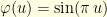 and
and

In other words, the random walk with increments conditioned to stay inside has probability transitions given by
Next section investigates the limiting case .
Conclusion
We have computed the dynamics of the conditioned random walk with space-increments  . To obtain the dynamics of the conditioned Brownian motion it suffices to consider the limiting case . The drift of the resulting diffusion is given by

The same computation gives the volatility of the resulting diffusion. It is given by

As the consequence, this shows that a Brownian motion conditioned to stay inside follows the stochastic differential equation 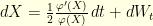 where
where  is the first eigenfunction of the Laplacian on with Dirichlet boundary conditions. More generaly, the same argument would show that a Brownian motion in
  conditioned to stay inside a nice bounded domain evolves according to the stochastic differential equation

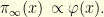
where  is the first eigenfunction of the Laplacian on . This is a Langevin diffusion and one can immediately see that the invariant distribution of this diffusion is given by
For example, the following plot depicts the first eigenfunction of the Laplacian on the domain ![{D=[0,1]^2 \subset \mathbb{R}^2}](https://s0.wp.com/latex.php?latex=%7BD%3D%5B0%2C1%5D%5E2+%5Csubset+%5Cmathbb%7BR%7D%5E2%7D&bg=ffffe3&fg=000000&s=0&c=20201002) .
.

First Eigenfunction


