June | 2011 | Journey into Randomness

Uncertainty Principle and Robust Reconstruction

June 12, 2011 at 11:42 pm (compressed sensing, Uncategorized)
Tags: compressed sensing, Heisenberg, Logan phenomenon, l^1, reconstruction, robust reconstruction, sparsity, uncertainty principle

1. Heisenberg Uncertainty Principle

The Heisenberg Uncertainty principle states that a signal cannot be both highly concentrated in time and highly concentrated in frequency. For example, consider a square-integrable function ${f:{\mathbb R} \rightarrow {\mathbb R}}$ normalised so that ${\|f\|_2 =1}$ . In this case, ${|f(x)|^2 \, dx}$ defines a probability distributions on the real line. The Fourier isometry shows that its Fourier transform ${\hat{f}}$ also defines a probability distribution ${|\hat{f}(x)|^2 \, dx}$ . In order to measure how spread-out these two probability distributions are, one can use their variance. The uncertainty principle states that

$\displaystyle \textbf{var}(|f|^2) \cdot \textbf{var}(|\hat{f}|^2) \geq \frac{1}{16\pi^2} \ \ \ \ \ (1)$

where ${\textbf{var}(g)}$ designates the variance of the distribution ${g(x) \, dx}$ . This shows for example that ${\textbf{var}(|f|^2)}$ and ${\textbf{var}(|\hat{f}|^2)}$ cannot be simultaneously less than ${\frac{1}{4 \pi}}$ .

We can play the same with a vector ${x \in {\mathbb R}^N}$ and its (discrete) Fourier transform ${\hat{x} = Hx}$ . The Fourier matrix ${H}$ is defined by

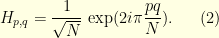
$\displaystyle H_{p,q} = \frac{1}{\sqrt{N}} \, \exp(2i\pi\frac{pq}{N}). \ \ \ \ \ (2)$

where the normalisation coefficient ${\frac{1}{\sqrt{N}}}$ ensures that ${HH_*=I}$ . The Fourier inversion formula reads ${x = H_*\hat{x}}$ . To measure how spread-out the coefficients of a vector ${v \in {\mathbb C}^N}$ are, one can look at the size of its support

$\displaystyle \mu(v) \, := \, \textbf{Card} \Big\{ k \in [1,N]: \; v_k=0 \Big\}. \ \ \ \ \ (3)$

If an uncertainty principle holds, one should be able to bound ${\mu(x) \cdot \mu(\hat{x})}$ from below. There is no universal constant ${\alpha>0}$ such that

$\displaystyle \frac{\mu(x)}{N} \cdot \frac{\mu(\hat{x})}{N} \geq \alpha \ \ \ \ \ (4)$

for any ${N \geq 1}$ and ${x \in {\mathbb R}^N}$ . Indeed, if ${N=pq}$ and ${x = \sum_{j=1}^{\frac{N}{p}} e_{pj}}$ one readily checks that ${\mu(x) = q}$ and ${\mu(\hat{x})=p}$ so that ${\frac{\mu(x)}{N} \cdot \frac{\mu(\hat{x})}{N} = \frac{1}{N}}$ . Nevertheless, in this case this gives ${\mu(x) \cdot \mu(\hat{x}) = N}$ . Indeed, a beautiful result of L. Donoho and B. Stark shows that

$\displaystyle \mu(x) \cdot \mu(\hat{x}) \geq N \qquad \text{for all } \qquad x \in {\mathbb R}^N. \ \ \ \ \ (5)$

Maybe more surprisingly, and crucial to applications, they even show that this principle can be made robust by taking noise and approximations into account. This is described in the next section.

2. Robust Uncertainty Principle

Consider a subset ${T \subset \{1,2, \dots, N\}}$ of indices and the orthogonal projection ${P_T}$ on ${\text{span}\big\{ e_t : t \in T\big\}}$ . In other words, if ${x = \sum_{j=1}^N x_j e_j}$ , then

$\displaystyle P_T x = \sum_{t \in T} x_t \, e_t. \ \ \ \ \ (6)$

We say that a vector ${x \in {\mathbb C}^N}$ is ${\epsilon_T}$ -concentrated on ${T}$ if ${\|x-P_T x\|_2 \leq \epsilon_T}$ . The ${\ell^2}$ -robust uncertainty principle states that if ${x}$ is ${\epsilon_T}$ concentrated on ${T}$ and ${\hat{x}}$ is ${\epsilon_W}$ -concentrated on ${W}$ then

$\displaystyle |T| \cdot |W| \geq N \, \big( 1 - \epsilon_2\big) \qquad \text{with} \qquad 1 - \epsilon_2 = \big(1-(\epsilon_W+\epsilon_W)\big)^2. \ \ \ \ \ (7)$

Indeed, the case ${\epsilon_T=\epsilon_W=0}$ gives Equation (5). The proof is surprisingly easy. On introduces the reconstruction operator ${R}$ defined by

$\displaystyle R = H_* \circ P_W \circ H \circ P_T. \ \ \ \ \ (8)$

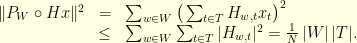
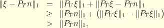
In words: take a vector, delete the coordinate outside ${T}$ , take the Fourier transform, delete the coordinate outside ${W}$ , finally take the inverse Fourier transform. The special case ${T=W=\{1,\ldots, N\}}$ simply gives ${R=\text{(identity)}}$ . The proof consists in bounding the operator norm of ${R: \ell^2 \rightarrow \ell^2}$ from above and below. The existence of a vector ${x}$ that is ${\epsilon_T}$ -concentrated such that ${\hat{x}}$ is ${\epsilon_W}$ -concentrated gives a lower bound. In details:

Upper bound: it is obvious that ${R}$ is a contraction in the sense that ${\|Rx\| \leq \|x\|}$ since ${H,H_*}$ are isometries and ${P_T,P_W}$ are orthogonal projections. Moreover, the smaller ${W}$ and ${T}$ , the smaller the norm of ${R}$ . Since ${H_*}$ is an isometry we have ${\|R\| = \|P_W \circ H \circ P_T\| = \sup \|P_W \circ H x\|}$ , where the supremum is over all ${\|x\| \leq 1}$ that are supported by ${T}$ . Cauchy-Schwarz shows that
$\displaystyle \begin{array}{rcl} \|P_W \circ H x\|^2 &=& \sum_{w \in W} \big( \sum_{t \in T} H_{w,t} x_t\big)^2 \\ &\leq& \sum_{w \in W} \sum_{t \in T} |H_{w,t}|^2 = \frac{1}{N}\,|W| \, |T|. \end{array}$

In other words, the reconstruction operator ${R}$ satisfies ${\|R\| \leq \frac{1}{\sqrt{N}}\, \sqrt{|W| \, |T|}}$ . This is a non-trivial bound only if ${|W| \, |T| < N}$ .
Lower bound: consider ${x \in {\mathbb R}^N}$ that satisfies ${\|x-P_Tx\| = \epsilon_T}$ and ${\|\hat{x} - P_W \hat{x}\| = \epsilon_W}$ . The Fourier transform is an ${\ell^2}$ isometry so that the triangle inequality easily shows that ${x \approx Rx}$ in the sense that
$\displaystyle \|x-R x\| \leq \epsilon_W + \epsilon_T. \ \ \ \ \ (9)$

This proves the lower bound ${\|R\| \geq 1-(\epsilon_W+\epsilon_T)}$ .

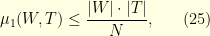
In summary, the reconstruction operator ${R=H_* \circ P_W \circ H \circ P_T}$ always satisfies ${\|R\| \leq \frac{1}{\sqrt{N}}\, \sqrt{|W| \, |T|}}$ . Moreover, the existence of ${x \in {\mathbb R}^N}$ satisfying ${\|x-P_Tx\|_2 = \epsilon_T}$ and ${\|\hat{x} - P_W \hat{x}\|_2 = \epsilon_W}$ implies the lower bound ${\|R\| \geq 1-(\epsilon_W+\epsilon_T)}$ . Therefore, the sets ${W}$ and ${T}$ must verify the uncertainty principle

$\displaystyle |W| \cdot |T| \geq N \, (1-\epsilon_2) \qquad \text{with}\qquad 1-\epsilon_2 = \big( 1-(\epsilon_W+\epsilon_T)\big)^2. \ \ \ \ \ (10)$

Notice that we have only use the fact that the entries of the Fourier matrix are bounded in absolute value by ${\frac{1}{\sqrt{N}}}$ . We could have use for example any other unitary matrix ${U \in M_N({\mathbb C})}$ . The bound ${|U_{r,s}| \leq \frac{1}{\sqrt{\alpha N}}}$ for all ${1 \leq r,s \leq N}$ gives the uncertainty principle ${|W| \cdot |T| \geq \alpha N \, \big( 1-(\epsilon_W+\epsilon_T)\big)^2}$ . In general ${\alpha \leq 1}$ since ${U}$ is an isometry.

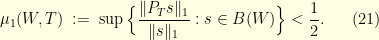
One can work out an upper bound and a lower bound for the reconstruction operator ${R}$ using the ${\ell^1}$ -norm instead of the ${\ell^2}$ -norm. Doing so, one can prove that if ${\|x-P_Tx\|_1 \leq \epsilon_T}$ and ${\|\hat{x}-P_W \hat{x}\|_1 \leq \epsilon_W}$ then

$\displaystyle |W| \cdot |T| \geq N \, (1-\epsilon_1) \qquad \text{with}\qquad 1-\epsilon_1 = \frac{1-(\epsilon_W+\epsilon_T)}{1+\epsilon_W}. \ \ \ \ \ (11)$

3. Stable ${\ell^2}$ Reconstruction

Let us see how the uncertainty principle can be used to reconstruct a corrupted signal. For example, consider a discrete signal ${\big\{ s_k \big\}_{k=1}^N}$ corrupted by some noise ${\big\{ n_k \big\}_{k=1}^N}$ . In top of that, let us suppose that on the set ${T \subset \{1,\ldots, N\}}$ the receiver does not receive any information. In other words, the receiver can only observe

$\displaystyle y_k = s_k + n_k \qquad \text{for} \qquad k \in \{1,\ldots, N\} \setminus T. \ \ \ \ \ (12)$

In general, it is impossible to recover the original ${s_k}$ , or an approximation of it, since the data ${s_k}$ for ${k \in T}$ are lost forever. In general, even if the received signal ${y_k}$ is very weak, the deleted data ${\{s_k\}_{k \in T}}$ might be huge. Nevertheless, under the assumption that the frequencies of ${s}$ are supported by a set ${W}$ satisfying ${|T| \cdot |W| < N}$ , the reconstruction becomes possible. It is not very surprising since the hypothesis ${|T| \cdot |W| < N}$ implies that the signal ${\{s_k\}_1^N}$ is sufficiently smooth so that the knowledge of ${y_k + n_k}$ on ${k \in \{1,\ldots, N\} \setminus T}$ is enough to construct an approximation of ${s_k}$ for ${k \in T}$ . We assume that the set ${W}$ is known to the observer. Since the components on ${T}$ are not observed, one can suppose without loss of generality that there is no noise on these components ( ${i.e.}$ we have ${n_k=0}$ for ${k \in T}$ ): the observation ${y}$ can be described as

$\displaystyle y = (I-P_T)s + n. \ \ \ \ \ (13)$

It is possible to have a stable reconstruction of the original signal ${s}$ if the operator ${(I-P_T)}$ can be inverted: there exists a linear operator ${Q}$ such that ${Q \circ (I-P_T) s = s}$ for every ${s \in B(W)}$ . If this is the case, the reconstruction

$\displaystyle \hat{s} = Q y \ \ \ \ \ (14)$

satisfies ${\hat{s} = s + Qn}$ so that ${\|\hat{s}-s\|_2 \leq \|Q\| \, \|n\|_2}$ . A sufficient condition for ${Q}$ to exist is that ${\|P_T s\| < \|s\|}$ for every ${s \in B(W)}$ . This is equivalent to

$\displaystyle \mu_2(W,T) \;:=\; \sup\Big\{ \frac{\|P_T s\|_2}{\|s\|_2}: s \in B(W)\Big\} < 1. \ \ \ \ \ (15)$

Since for ${s \in B(W)}$ we have ${s = (H_* \circ P_W \circ H) s}$ it follows that ${P_T s = R^* \, s}$ where ${R=H_* \circ P_W \circ H \circ P_T}$ is the reconstruction operator. The condition ${\mu_2(W,F) < 1}$ thus follows from the bound ${\|R\| \leq \sqrt{\frac{|T| \cdot |W|}{N}}<1}$ . Consequently the operator ${(I-P_T)}$ is invertible since ${Q=(1-R^*)^{-1}}$ satisfies

$\displaystyle Q \circ (1-P_T) s=s \qquad \text{for all} \qquad s \in B(W). \ \ \ \ \ (16)$

Since ${\|Q\| = \|(1-R^*)^{-1}\| \leq (1-\|R\|)^{-1}}$ we have the bound ${\|Q\| \leq C = (1-\frac{|W| \cdot |T|}{N})^{-1}}$ . Therefore

$\displaystyle \text{(error reconstruction)} = \| \hat{s}-s\|_2 \leq C \, \|n\|_2. \ \ \ \ \ (17)$

Notice also that ${\hat{s} = Q y}$ can easily and quickly be approximated using the expansion

$\displaystyle Q = (1-R^*)^{-1}= 1 + R^* + (R^*)^2 + (R^*)^3 + \ldots \ \ \ \ \ (18)$

Nevertheless, there are two things that are not very satisfying:

the bound ${|W| \cdot |T| < N}$ is extremely restrictive. For example, if ${10 \%}$ of the component are corrupted, this imposes that the signal has only ${10}$ (and not ${10\%}$ ) non-zero Fourier coefficients.
in general, the sets ${W}$ and ${T}$ are not known by the receiver.

The theory of compressed sensing addresses these two questions. More on that in forthcoming posts, hopefully … Emmanuel Candes recently gave extremely interesting lectures on compressed sensing.

4. Exact ${\ell^1}$ Reconstruction: Logan Phenomenon

Let us consider a slightly different situation. A small fraction of the components of a signal ${\{s_k\}_{k=1}^N}$ are corrupted. The noise is not assumed to be small. More precisely, suppose that one observes

$\displaystyle y_k = s_k + P_T n_k \ \ \ \ \ (19)$

where ${T}$ is the set of corrupted components and ${n}$ is an arbitrary noise that can potentially have very high intensity. Moreover, the set ${T}$ is unknown to the receiver. In general, it is indeed impossible to recover the original signal ${s}$ . Surprisingly, if one assumes that the signal ${s}$ is band-limited ${i.e.}$ the Fourier transform of ${s}$ is supported by a known set ${W}$ that satisfies

$\displaystyle |W| \cdot |T| < \frac{N}{2}, \ \ \ \ \ (20)$

it is possible to recover exactly the original ${s}$ . The main argument is that the condition (20) implies that the signal ${s}$ has more that ${50\%}$ of its energy on ${U=T^c}$ in the sense that ${\|P_U s\|_1> \|P_{T} s\|_1}$ . Consequently, since ${U}$ is the set where the signal ${s}$ is perfectly known, enough information is available to recover the original signal ${s}$ . To prove the inequality ${\|P_U s\|_1> \|P_{T} s\|_1}$ , it suffices to check that

$\displaystyle \mu_1(W,T) \;:=\; \sup\Big\{ \frac{\|P_T s\|_1}{\|s\|_1}: s \in B(W)\Big\} < \frac{1}{2}. \ \ \ \ \ (21)$

In this case we have ${\|P_U\ s\|_1 = \|s\|_1 - \|P_T s\|_1 > \frac{1}{2} \|s\| > \|P_T s\|_1}$ , which prove that ${s}$ has more that ${50\%}$ of its energy on ${U}$ . Indeed, the same conclusion holds with the ${\ell^2}$ -norm if the condition ${\mu_2(W,T) < \frac12}$ holds. The magic of the ${\ell^1}$ -norm is that condition ${\mu_1(W,T) < \frac12}$ implies that the signal ${s}$ is solution of the optimisation problem

$\displaystyle s \;=\; \textbf{argmin} \big\{ \|\tilde{s} - y\|_1 : \tilde{s} \in B(W) \Big\}. \ \ \ \ \ (22)$

This would not be true if one were using the ${\ell^2}$ norm instead. This idea was first discovered in a slightly different context in Logan’s thesis (1965). More details here. To prove (22), notice that any ${\tilde{s} \in B(W)}$ can be written as ${\tilde{s}= s+\xi}$ with ${\xi \in B(W)}$ . Therefore, since ${\tilde{s} - y = \xi - P_T n}$ , it suffices to show that

$\displaystyle 0 = \textbf{argmin} \big\{ \| \xi - P_T n\|_1 : \xi \in B(W) \Big\}. \ \ \ \ \ (23)$

This is equivalent to proving that for any non-zero ${\xi \in B(W)}$ we have

$\displaystyle \| \xi - P_T n\|_1 > \|P_T n\|_1. \ \ \ \ \ (24)$

It is now that the ${\ell^1}$ -norm is crucial. Indeed, we have

$\displaystyle \begin{array}{rcl} \| \xi - P_T n\|_1 &=& \|P_U \xi\|_1 + \| P_T \xi - P_T n\|_1 \\ &\geq& \|P_T n\|_1 + \big( \|P_U \xi\|_1- \|P_{T} \xi\|_1\big)\\ &>& \|P_T n\|_1, \end{array}$

which gives the conclusion. This would not work for any ${\ell^p}$ -norm with ${p>1}$ since in general ${\| \xi - P_T n\|_r \geq \|P_U \xi\|_r + \| P_T \xi - P_T n\|_r}$ : the inequality is in the wrong sense. In summary, as soon as the condition ${\mu_1(W,T) < \frac{1}{2}}$ is satisfied, one can recover the original signal by solving the ${\ell^1}$ minimisation problem (22).

\noindent Because it is not hard to check that in general we always have

$\displaystyle \mu_1(W,T) \leq \frac{|W| \cdot |T|}{N}, \ \ \ \ \ (25)$

this shows that the condition ${|W| \cdot |T| < \frac{N}{2}}$ implies that exact recovery is possible! Nevertheless, the condition ${\mu_1(W,T) \leq \frac{|W| \cdot |T|}{N}}$ is far from satisfying. The inequality is tight but in practice it happens very often that ${\mu_1(W,T) < \frac{1}{2}}$ even if ${|W| \cdot |T|}$ is much bigger that ${\frac{N}{2}}$ .

The take away message might be that perfect recovery is often possible if the signal has a sparse representation in an appropriate basis (in the example above, the usual Fourier Basis): the signal can then be recovered by ${\ell^1}$ -minimisation. For this to be possible, the representation basis (here the Fourier basis) must be incoherent with the observation basis in the sense that the coefficients of the change of basis matrix (here, Fourier matrix) must be small ${i.e.}$ if ${(e_1, \ldots, e_N)}$ is the observation basis and ${(\hat{e}_1, \ldots, \hat{e}_N)}$ is the representation basis then ${\langle e_i, \hat{e}_j \rangle}$ must be small for every ${1 \leq i,j \leq N}$ . For example, for the Fourier basis we have ${|\langle e_i, \hat{e}_j \rangle| = \frac{1}{\sqrt{N}}}$ for every ${1 \leq i,j \leq N}$ .