Recently, Yann Ollivier developed a nice theory of Ricci curvature for Markov chains. In many ways, this can be seen as a geometric language giving another view on the notion of path coupling, developed at the end of the  ‘s by Martin Dyer and co-workers. It has to be noted that this new notion of curvature is very general and does not need the state space where the Markov chain evolves to have any differential structure, as can be expected at first sight. Any state space endowed with a metric suffices.
Let  be a Markov kernel on a metric state space
  . We would like to quantify how long it takes for two different particles evolving according to the Markovian dynamic given by to meet. If the first particle starts at
  and the second at
  , the initial distance between them is
  . At time
  , what is the average distance between these two particles. For example, if
  and
and  are two Brownian motions in
  started from
  and
and  respectively, there is no reason why
  and
and  should be closer from each other than
  and
and  . Indeed, one can even show that whatever the coupling of these two Brownian motions we have
 ![{\mathop{\mathbb E}[d(W^x_t, W^y_t)] \geq d(x,y)}](https://s0.wp.com/latex.php?latex=%7B%5Cmathop%7B%5Cmathbb+E%7D%5Bd%28W%5Ex_t%2C+W%5Ey_t%29%5D+%5Cgeq+d%28x%2Cy%29%7D&bg=ffffe3&fg=000000&s=0&c=20201002) : this is roughly speaking because the Euclidean space has no curvature. The situation is quite different if we were instead considering Brownian motions on a sphere: in this case, trajectories tend to coalesce.
: this is roughly speaking because the Euclidean space has no curvature. The situation is quite different if we were instead considering Brownian motions on a sphere: in this case, trajectories tend to coalesce.
1. Wasserstein distance
In the sequel, we will need to use a notion of distance between probability distributions on the metric space . The usual total variation distance  defined by

is not adapted to our purpose since the metric structure of the space is not exploited. Instead, in order to take into account the distance  of the space
  and develop a notion of curvature, we use the Wasserstein distance
  between probability measures. It is defined as

The distance is crucial to this definition: a change of distance implies a change of the class of  -Lipschitz functions. Since
 ![{\mu(f) - \nu(f) = \mathop{\mathbb E}[f(X) - f(Y)]}](https://s0.wp.com/latex.php?latex=%7B%5Cmu%28f%29+-+%5Cnu%28f%29+%3D+%5Cmathop%7B%5Cmathbb+E%7D%5Bf%28X%29+-+f%28Y%29%5D%7D&bg=ffffe3&fg=000000&s=0&c=20201002) for any coupling
for any coupling  of
of  and
and  , and since the function
  is -Lipschitz, it follows that
 ![{\mathop{\mathbb E}[f(X) - f(Y)] \leq \mathop{\mathbb E}[d(X,Y)]}](https://s0.wp.com/latex.php?latex=%7B%5Cmathop%7B%5Cmathbb+E%7D%5Bf%28X%29+-+f%28Y%29%5D+%5Cleq+%5Cmathop%7B%5Cmathbb+E%7D%5Bd%28X%2CY%29%5D%7D&bg=ffffe3&fg=000000&s=0&c=20201002) . Consequently, for any coupling we have
. Consequently, for any coupling we have ![{W(\mu,\nu) \leq \mathop{\mathbb E}[d(X,Y)]}](https://s0.wp.com/latex.php?latex=%7BW%28%5Cmu%2C%5Cnu%29+%5Cleq+%5Cmathop%7B%5Cmathbb+E%7D%5Bd%28X%2CY%29%5D%7D&bg=ffffe3&fg=000000&s=0&c=20201002) . Taking the infimum over all the couplings leads to the inequality
. Taking the infimum over all the couplings leads to the inequality
![\displaystyle W(\mu,\nu) \;=\; \sup_{\text{Lip}(f) \leq 1} \; |\mu(f) - \nu(f)| \;\leq\; \inf_{(X,Y)} \; \mathop{\mathbb E}[d(X,Y)]. \ \ \ \ \ (3)](https://s0.wp.com/latex.php?latex=%5Cdisplaystyle++W%28%5Cmu%2C%5Cnu%29+%5C%3B%3D%5C%3B+%5Csup_%7B%5Ctext%7BLip%7D%28f%29+%5Cleq+1%7D+%5C%3B+%7C%5Cmu%28f%29+-+%5Cnu%28f%29%7C+%5C%3B%5Cleq%5C%3B+%5Cinf_%7B%28X%2CY%29%7D+%5C%3B+%5Cmathop%7B%5Cmathbb+E%7D%5Bd%28X%2CY%29%5D.+%5C+%5C+%5C+%5C+%5C+%283%29&bg=ffffe3&fg=000000&s=0&c=20201002)
This is a deep result that on any reasonable space the inequality is in fact an equality. Indeed, Kantorovich duality states that on any Radon space we have
![\displaystyle W(\mu,\nu) \;=\; \sup_{\text{Lip}(f) \leq 1} \; |\mu(f) - \nu(f)| \;=\; \inf_{(X,Y)} \; \mathop{\mathbb E}[d(X,Y)]. \ \ \ \ \ (4)](https://s0.wp.com/latex.php?latex=%5Cdisplaystyle+++W%28%5Cmu%2C%5Cnu%29+%5C%3B%3D%5C%3B+%5Csup_%7B%5Ctext%7BLip%7D%28f%29+%5Cleq+1%7D+%5C%3B+%7C%5Cmu%28f%29+-+%5Cnu%28f%29%7C+%5C%3B%3D%5C%3B+%5Cinf_%7B%28X%2CY%29%7D+%5C%3B+%5Cmathop%7B%5Cmathbb+E%7D%5Bd%28X%2CY%29%5D.+%5C+%5C+%5C+%5C+%5C+%284%29&bg=ffffe3&fg=000000&s=0&c=20201002)
It is interesting to note that under mild conditions on the state space one can always find a coupling that achieves the infimum of (4): this is an easy compactness argument.
2. Notion of Curvature
Denoting by  the one step distribution of the Markov chain started from in the sense that
 ![{m_x(A) = \mathop{\mathbb P}[X_1 \in A \;| X_0 = x ]}](https://s0.wp.com/latex.php?latex=%7Bm_x%28A%29+%3D+%5Cmathop%7B%5Cmathbb+P%7D%5BX_1+%5Cin+A+%5C%3B%7C+X_0+%3D+x+%5D%7D&bg=ffffe3&fg=000000&s=0&c=20201002) , we define the local (Ricci) curvature
, we define the local (Ricci) curvature  between and as

The closer to is  , the more the trajectories started at tend to meet the trajectories started at .

Trajectories tend to coalesce
The interesting case is when the infimum  is strictly positive,

In this case we say that the Markov kernel is positively curved on . It should be noted that in many natural spaces it suffices to ensure that  for all neighbouring states and to ensure that for any pair
  . This can be proved thanks to the so called Gluing Lemma. A space without curvature correspond to the case
  : for example, a symmetric random walk on
  and a Brownian motion on
  have both zero curvature. The curvature
  is a property of both the metric space and the Markov kernel : indeed, different Markov chain on the same metric space have generally different associated curvature. Given a metric space carrying a probability distribution
  , this is an interesting problem to construct a -invariant Markov chain with the highest possible curvature .
Indeed, the notion of curvature readily generalizes to continuous time Markov processes by taking a limiting case of (5). For example, one can define the curvature of the continuous time Markov process  as the largest real number such that for any
  and
and  we have

for every  small enough. The quantity
  is the distribution of
  when started from in the sense that
 ![{m_x^{\delta}(A) = \mathop{\mathbb P}[X_{\delta} \in A \; |X_0=x]}](https://s0.wp.com/latex.php?latex=%7Bm_x%5E%7B%5Cdelta%7D%28A%29+%3D+%5Cmathop%7B%5Cmathbb+P%7D%5BX_%7B%5Cdelta%7D+%5Cin+A+%5C%3B+%7CX_0%3Dx%5D%7D&bg=ffffe3&fg=000000&s=0&c=20201002) .
.
3. Contraction property
We now show that a positive curvature implies a contraction property. Equation (5) shows that  for any . A simple argument shows that one can indeed generalize the situation to any two distributions
  in the sense that

Proof: For any pair consider a coupling  of
of  and
and  such that
 ![{W(m_x,m_y)=\mathop{\mathbb E}[d(U_{x,y}, V_{x,y})]}](https://s0.wp.com/latex.php?latex=%7BW%28m_x%2Cm_y%29%3D%5Cmathop%7B%5Cmathbb+E%7D%5Bd%28U_%7Bx%2Cy%7D%2C+V_%7Bx%2Cy%7D%29%5D%7D&bg=ffffe3&fg=000000&s=0&c=20201002) . Now, choose an optimal coupling of and . This is straightforward to check that
. Now, choose an optimal coupling of and . This is straightforward to check that  is a coupling (in general not optimal) of
  and
and  so that
![\displaystyle \begin{array}{rcl} W(\mu P, \nu P) &\leq& \mathop{\mathbb E}[d(U_{X,Y}, V_{X,Y})] = \mathop{\mathbb E}[\; \mathop{\mathbb E}[d(U_{x,y}, V_{x,y}) \;|X=x, Y=y] ] \\ &=& \mathop{\mathbb E}[ W(m_X, m_Y) ] = \mathop{\mathbb E}[ d(X,Y) \cdot (1-\kappa(X,Y)) ]\\ &\leq& (1-\kappa) \; \mathop{\mathbb E}[ d(X,Y) ] = (1-\kappa) \; W(\mu,\nu). \end{array}](https://s0.wp.com/latex.php?latex=%5Cdisplaystyle++%5Cbegin%7Barray%7D%7Brcl%7D++W%28%5Cmu+P%2C+%5Cnu+P%29+%26%5Cleq%26+%5Cmathop%7B%5Cmathbb+E%7D%5Bd%28U_%7BX%2CY%7D%2C+V_%7BX%2CY%7D%29%5D+%3D+%5Cmathop%7B%5Cmathbb+E%7D%5B%5C%3B+%5Cmathop%7B%5Cmathbb+E%7D%5Bd%28U_%7Bx%2Cy%7D%2C+V_%7Bx%2Cy%7D%29+%5C%3B%7CX%3Dx%2C+Y%3Dy%5D+%5D+%5C%5C+%26%3D%26+%5Cmathop%7B%5Cmathbb+E%7D%5B+W%28m_X%2C+m_Y%29+%5D+%3D+%5Cmathop%7B%5Cmathbb+E%7D%5B+d%28X%2CY%29+%5Ccdot+%281-%5Ckappa%28X%2CY%29%29+%5D%5C%5C+%26%5Cleq%26+%281-%5Ckappa%29+%5C%3B+%5Cmathop%7B%5Cmathbb+E%7D%5B+d%28X%2CY%29+%5D+%3D+%281-%5Ckappa%29+%5C%3B+W%28%5Cmu%2C%5Cnu%29.+%5Cend%7Barray%7D+&bg=ffffe3&fg=000000&s=0&c=20201002)

Equation (8) is extremely powerful since it immediately shows that

In other words, there is exponential convergence (in the Wasserstein metric) to the invariance distribution at rate  . In continuous time, this reads

In other words, the higher the curvature, the faster the convergence to equilibrium.
4. Examples
Let us give examples of positively curved Markov chains.
- Langevin diffusion with convex potential: consider a convex potential
 that is uniformly elliptic in the sense
  . The Langevin diffusion
  has invariant distribution with density proportional to
  . Given a time step , the Euler discretization of this diffusion reads

where  . Given two starting points
  and
and  , using the same noise
  to define
  and
and  it immediately follows that

In other words, the Langevin diffusion  is positively curved with curvature (at least) equal to
  .
.
- Brownian motion on a sphere: consider a Brownian motion on the unit sphere of . Consider two points
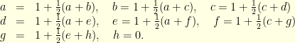
 on this unit sphere: by symmetry, one can always rotate the coordinates so that that
  and
and  for some
 ![{h \in [0,1]}](https://s0.wp.com/latex.php?latex=%7Bh+%5Cin+%5B0%2C1%5D%7D&bg=ffffe3&fg=000000&s=0&c=20201002) . For
. For  the (geodesic) distance
  is approximated by
  . One can couple two Brownian motions
  and
and  , one started at
  and the other one started at
  , by the usual symmetry with respect to the plane
  : in other words, is the reflexion of with respect to
  . One can check (good exercise!) that the diffusion followed by the
  -coordinate of a Brownian motion on the unit sphere of is simply given by
With this coupling, for small time  , it follows that

where is used as the same source of randomness for  and
and  since is the reflexion of . Since
  it readily follows that

In other words, the curvature of a Brownian motion on the unit sphere of is equal to  . Maybe surprisingly, the higher the dimension, the faster the convergence to equilibrium. This is not so unreal if one notices that the Brownian increment satisfies
  .
.
- Other examples: see the original text for many other examples.


![{\mathbb{E}[M_{\tau}] = 0}](https://s0.wp.com/latex.php?latex=%7B%5Cmathbb%7BE%7D%5BM_%7B%5Ctau%7D%5D+%3D+0%7D&bg=ffffe3&fg=000000&s=0&c=20201002)


![{\mathbb{E}[\tau] = \sum_{j=0}^{\tau-1} 2^{\tau-k} \, \delta_j}](https://s0.wp.com/latex.php?latex=%7B%5Cmathbb%7BE%7D%5B%5Ctau%5D+%3D+%5Csum_%7Bj%3D0%7D%5E%7B%5Ctau-1%7D+2%5E%7B%5Ctau-k%7D+%5C%2C+%5Cdelta_j%7D&bg=ffffe3&fg=000000&s=0&c=20201002)


![{\mathbb{E}[\tau] = 2^1+2^4+2^7}](https://s0.wp.com/latex.php?latex=%7B%5Cmathbb%7BE%7D%5B%5Ctau%5D+%3D+2%5E1%2B2%5E4%2B2%5E7%7D&bg=ffffe3&fg=000000&s=0&c=20201002)


 and compose with random transpositions: in short, at time
  where
where  is a transposition chosen uniformly at random among the
  transpositions of
  , where
  is a fixed constant ?
 steps to see this giant cycle! The first half of the proof is such a beauty that I cannot resist in sharing it here!
 that sends
  etc… It can be graphically represented by the following pictures:
 , this gives the following cycle structure:
 this gives,
 can be obtained from the cycle structure of
  in only 2 ways:
 behaves like a fragmentation-coalescence processes. At the beginning, the cycle structure of
  is trivial: there are
  trivial cycles of length one! Then, as times goes by, they begin to merge, and sometimes they also break down. At each step two integers
  and
and  are chosen uniformly at random (with
  ): if
): if  .
. where
where  : this graph has
  . A coupling argument makes this idea more precise:
 and the graph

 , take
  .
. is one of the most studied object: it is well-known that for
  , with probability tending to
  is of order
  . Since
  , this immediately shows that for
  , with
  the length of the longuest cycle in
  , the first cycle of order
  with cycle decomposition
  (cycles of length
 that measures in some extends the sizes of the cycles. In order to normalize everything and to take into account that the cycle structure abruptly changes near the critical value
 lies between
  and
and 
 between time
  and
and  for dimensions
  .
. converge (in probability) towards a non trivial constant
  ? It must be the analogue quantity for the random graph
  , so I bet it is a known result …
