I would like to discuss in this post the importance of the heuristic functional
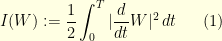
that often shows up when doing analysis on the Wiener space ![{S = (C([0,T], {\mathbb R}), \|\cdot\|_{\infty})}](https://s0.wp.com/latex.php?latex=%7BS+%3D+%28C%28%5B0%2CT%5D%2C+%7B%5Cmathbb+R%7D%29%2C+%5C%7C%5Ccdot%5C%7C_%7B%5Cinfty%7D%29%7D&bg=ffffe3&fg=000000&s=0&c=20201002) : an element of the Wiener space is traditionally denoted by
: an element of the Wiener space is traditionally denoted by  – this is a continuous function and
  is its value at time
 ![{t \in [0,T]}](https://s0.wp.com/latex.php?latex=%7Bt+%5Cin+%5B0%2CT%5D%7D&bg=ffffe3&fg=000000&s=0&c=20201002) . For a (nice) subset
. For a (nice) subset  of
of  , the Wiener measure of is nothing else than the probability that a Brownian path belongs to . Having said that, the quantity
  hardly makes sense since a Brownian path
 ![{(W_t: t \in [0,T])}](https://s0.wp.com/latex.php?latex=%7B%28W_t%3A+t+%5Cin+%5B0%2CT%5D%29%7D&bg=ffffe3&fg=000000&s=0&c=20201002) is (almost surely) non differentiable anywhere: still, this is a very useful heuristic in many situations. A review of probability can be found on the excellent blog of Terry Tao.
is (almost surely) non differentiable anywhere: still, this is a very useful heuristic in many situations. A review of probability can be found on the excellent blog of Terry Tao.
Where does it come from ?
As often, this is very instructive to come back to the discrete setting. Consider a time interval ![{[0,T]}](https://s0.wp.com/latex.php?latex=%7B%5B0%2CT%5D%7D&bg=ffffe3&fg=000000&s=0&c=20201002) and a discretization parameter
and a discretization parameter  : a discrete Brownian path is represented by the
  -tuple

The random variables  are independent centred Gaussian variables with variance
  so that the random vector
  has a density
  with respect to the -dimensional Lebesgue measure

The functional  is indeed a discretization of
  . Informally, the Wiener measure has a density proportional to
  with respect to the “infinite dimensional Lebesgue measure”: this does not make much sense because there is no such thing as the infinite dimensional Lebesgue measure. This should be understood as the limiting case
  of the discretization procedure presented above. Indeed, this is not an absolute non-sense to say that
![\displaystyle \mathop{\mathbb P}[ \omega = g] \sim e^{-I(g)}. \ \ \ \ \ (2)](https://s0.wp.com/latex.php?latex=%5Cdisplaystyle+%5Cmathop%7B%5Cmathbb+P%7D%5B+%5Comega+%3D+g%5D+%5Csim+e%5E%7B-I%28g%29%7D.+%5C+%5C+%5C+%5C+%5C+%282%29&bg=ffffe3&fg=000000&s=0&c=20201002)
because we will see that if  are two nice functions then
![\displaystyle \lim_{ \epsilon \rightarrow 0} \frac{P[ \|W-f\|_{\infty} < \epsilon]}{P[ \|W-g\|_{\infty} < \epsilon]} = \frac{e^{-I(f)}}{e^{-I(g)}}.](https://s0.wp.com/latex.php?latex=%5Cdisplaystyle+%5Clim_%7B+%5Cepsilon+%5Crightarrow+0%7D+%5Cfrac%7BP%5B+%5C%7CW-f%5C%7C_%7B%5Cinfty%7D+%3C+%5Cepsilon%5D%7D%7BP%5B+%5C%7CW-g%5C%7C_%7B%5Cinfty%7D+%3C+%5Cepsilon%5D%7D+%3D+%5Cfrac%7Be%5E%7B-I%28f%29%7D%7D%7Be%5E%7B-I%28g%29%7D%7D.&bg=ffffe3&fg=000000&s=0&c=20201002)
It is then very convenient to write
![\displaystyle \mathop{\mathbb P}[\omega \in A] = \int_{A} e^{-I(W)} \, d\lambda(W)](https://s0.wp.com/latex.php?latex=%5Cdisplaystyle+%5Cmathop%7B%5Cmathbb+P%7D%5B%5Comega+%5Cin+A%5D+%3D+%5Cint_%7BA%7D+e%5E%7B-I%28W%29%7D+%5C%2C+d%5Clambda%28W%29&bg=ffffe3&fg=000000&s=0&c=20201002)
where  is a fictional infinite dimensional Lebesgue measure (ie: translation invariant).
Translations in the Wiener space
As a first illustration of the heuristic ![{\mathop{\mathbb P}[\omega = g] \sim e^{-I(g)}}](https://s0.wp.com/latex.php?latex=%7B%5Cmathop%7B%5Cmathbb+P%7D%5B%5Comega+%3D+g%5D+%5Csim+e%5E%7B-I%28g%29%7D%7D&bg=ffffe3&fg=000000&s=0&c=20201002) , let see how the Wiener measure behave under translations. If we choose a nice continuous function
, let see how the Wiener measure behave under translations. If we choose a nice continuous function  such that
  is well defined (ie:
 ![{\dot{f} \in L^2([0,T]))}](https://s0.wp.com/latex.php?latex=%7B%5Cdot%7Bf%7D+%5Cin+L%5E2%28%5B0%2CT%5D%29%29%7D&bg=ffffe3&fg=000000&s=0&c=20201002) ), a translated probability measure
), a translated probability measure  can be defined through the relation

This is not clear that  is absolutely continuous with respect to the Wiener measure
  . Of course, we impose that
  . For a set
  , the heuristic says that

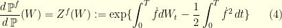
This is why, writing  , we obtain the following change of probability formula
Proposition 1 Cameron-Martin-Girsanov change of probability formula:
for any continuous function such that and ![{\dot{f} \in L^2([0,T])}](https://s0.wp.com/latex.php?latex=%7B%5Cdot%7Bf%7D+%5Cin+L%5E2%28%5B0%2CT%5D%29%7D&bg=ffffe3&fg=000000&s=0&c=20201002) ,
,
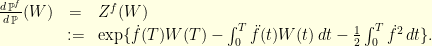
This change of probability formula is extremely useful since this is typically much more convenient to work with a Brownian motion  than with a drifted Brownian motion
  . In many situations, we get rid of the annoying stochastic integral
  : if is regular enough (
![{f \in C^3([0,T])}](https://s0.wp.com/latex.php?latex=%7Bf+%5Cin+C%5E3%28%5B0%2CT%5D%29%7D&bg=ffffe3&fg=000000&s=0&c=20201002) , say) we have
, say) we have
The next section is a straightforwards application of this change of variable formula.
Probability to be in an  -tube
-tube
Suppose that are two nice functions (smooth, say): for small  , what is a good approximation of the quotient
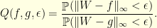
In words, this basically asks the question: how more probable is the event  than the event
  ? Of course, since this can also be read as
where  indicates the function identically equal to zero, it suffices to consider the case
  . If we introduce the event

the quotient  is equal to
  . This why, using the change of probability formula (4),
![\displaystyle \begin{array}{rcl} Q(f,0,\epsilon) &=& \frac{\mathop{\mathbb P}^f(A_{\epsilon})}{\mathop{\mathbb P}(A_{\epsilon})} = \frac{\mathop{\mathbb E}\left[ 1_{A_{\epsilon}}(W) Z^f(W) \right]}{\mathop{\mathbb E}\left[ 1_{A_{\epsilon}}(W) \right]} \end{array}](https://s0.wp.com/latex.php?latex=%5Cdisplaystyle+%5Cbegin%7Barray%7D%7Brcl%7D+Q%28f%2C0%2C%5Cepsilon%29+%26%3D%26+%5Cfrac%7B%5Cmathop%7B%5Cmathbb+P%7D%5Ef%28A_%7B%5Cepsilon%7D%29%7D%7B%5Cmathop%7B%5Cmathbb+P%7D%28A_%7B%5Cepsilon%7D%29%7D+%3D+%5Cfrac%7B%5Cmathop%7B%5Cmathbb+E%7D%5Cleft%5B+1_%7BA_%7B%5Cepsilon%7D%7D%28W%29+Z%5Ef%28W%29+%5Cright%5D%7D%7B%5Cmathop%7B%5Cmathbb+E%7D%5Cleft%5B+1_%7BA_%7B%5Cepsilon%7D%7D%28W%29+%5Cright%5D%7D+%5Cend%7Barray%7D+&bg=ffffe3&fg=000000&s=0&c=20201002)
with  . If
. If  , this is clear that for
  ,
,

Both sides going to zero when goes to zero, this is enough to conclude that

In short, for any two reasonably nice functions (for example ![{f,g \in C^3([0,T])}](https://s0.wp.com/latex.php?latex=%7Bf%2Cg+%5Cin+C%5E3%28%5B0%2CT%5D%29%7D&bg=ffffe3&fg=000000&s=0&c=20201002) ) that satisfy
) that satisfy  ,
,

Large deviation result
Take a subset of (it might be useful to think of sets like  ). We are interested to the probability that the rescaled (in space) Brownian motion

belongs to when goes to . Typically, if the null function does not belong to (the closure of) , the probability  is exponentially small. It turns out that if is regular enough

Again, the usual heuristic gives this result in no time if we accept not to be too rigorous:

This is very fishy since the Jacobian should behave very badly (actually the measure ![{\mathop{\mathbb P}[W \in \cdot]}](https://s0.wp.com/latex.php?latex=%7B%5Cmathop%7B%5Cmathbb+P%7D%5BW+%5Cin+%5Ccdot%5D%7D&bg=ffffe3&fg=000000&s=0&c=20201002) and
and ![{\mathop{\mathbb P}[\epsilon W \in \cdot]}](https://s0.wp.com/latex.php?latex=%7B%5Cmathop%7B%5Cmathbb+P%7D%5B%5Cepsilon+W+%5Cin+%5Ccdot%5D%7D&bg=ffffe3&fg=000000&s=0&c=20201002) are mutually singular) but all this mess can be made perfectly rigorous. Nevertheless, the basic idea is almost there, and it can be proved (Freidlin-Wentzel theory) that for any open set
are mutually singular) but all this mess can be made perfectly rigorous. Nevertheless, the basic idea is almost there, and it can be proved (Freidlin-Wentzel theory) that for any open set  ,
,

while for any closed set  ,
,

One cleaner way to prove this is to used the usual Cramer theorem of large deviations for sums of i.i.d random variables (in Banach space) and notice that for  then
then

where  are independent standard Brownian motions. Cramer theorem states that
![\displaystyle \mathop{\mathbb P}[ \frac{W_1+W_2+\ldots+W_N}{N} \in A] \sim \exp\{-N \inf\{I(f): f \in A\} \}](https://s0.wp.com/latex.php?latex=%5Cdisplaystyle+%5Cmathop%7B%5Cmathbb+P%7D%5B+%5Cfrac%7BW_1%2BW_2%2B%5Cldots%2BW_N%7D%7BN%7D+%5Cin+A%5D+%5Csim+%5Cexp%5C%7B-N+%5Cinf%5C%7BI%28f%29%3A+f+%5Cin+A%5C%7D+%5C%7D&bg=ffffe3&fg=000000&s=0&c=20201002)
with
![\displaystyle I(f) = \sup\{ \int_{0}^t f(t)g(t)\, dt - \ln \, \mathop{\mathbb E} e^{ \int_0^T g(t) W(t) \, dt } : g \in L^2([0,T])\}.](https://s0.wp.com/latex.php?latex=%5Cdisplaystyle+I%28f%29+%3D+%5Csup%5C%7B+%5Cint_%7B0%7D%5Et+f%28t%29g%28t%29%5C%2C+dt+-+%5Cln+%5C%2C+%5Cmathop%7B%5Cmathbb+E%7D+e%5E%7B+%5Cint_0%5ET+g%28t%29+W%28t%29+%5C%2C+dt+%7D+%3A+g+%5Cin+L%5E2%28%5B0%2CT%5D%29%5C%7D.&bg=ffffe3&fg=000000&s=0&c=20201002)
This is not very hard to see that the supremum is indeed  .
.

